To make an Excel drop-down list, select the cells, open the Data tab, click Data Validation, set Allow to List, and in Source either type the options separated by commas or select the cells that hold them. Click OK and each cell gets an arrow. It works the same way in Excel for Windows, Excel for Mac and the free Excel for the web.
That takes two minutes. The rest of this guide covers the version that keeps itself up to date, a second list that changes with the first, what to do when you need more than one choice per cell, and the fixes for the usual snags. Every step was checked against Microsoft's documentation for each platform on September 27, 2026.
Excel drop-down list sources at a glance
A drop-down list gets its options from one of four places. Which one you pick decides how much work editing the list is later.
Source | What you put in the Source box | Updates itself when you add options? | Best for |
|---|---|---|---|
Typed list |
| No, you edit the box | Short lists that rarely change |
Range of cells |
| No, you reselect the range | A list on another sheet |
Named range |
| No, you update the name | The same list on many sheets, and dependent lists |
Excel table | The table's column, selected with the mouse | Yes | Lists that grow |
Excel drop-down list examples
Three lists cover most of what people build, and each one is a few minutes' work with the steps below.
A status column: Not started, In progress, Blocked, Done. Pair it with the color rules further down and a COUNTIF to total each status.
A yes/no column: a typed list of
Yes,No. Quicker to fill than free text, and it never collects "Y", "yes" and "YES" in the same column.A category and an item: pick Fruit in one cell and the next cell offers only fruit. That is the dependent list, built with two named ranges and INDIRECT.
How do you create a drop-down list in Excel?
These are the steps from Microsoft's guide for Excel on Windows, with the parts people trip on filled in.
Type the options somewhere. A column on a second sheet keeps them out of the way. Leave the header out of the list, or "Status" turns up as a choice.
Select the cells that should get the list. Select the whole column of a table, or a range such as C2:C100, so you set it up once.
On the Data tab, click Data Validation.
On the Settings tab, set Allow to List.
Click in Source, then select the cells that hold your options. Or type them straight in, separated by commas and with no spaces after the commas, as Microsoft puts it: each item "separated by a comma, with no spaces in between".
Leave Ignore blank ticked if people may leave the cell empty, and keep In-cell dropdown ticked. That box is the arrow.
Click OK.
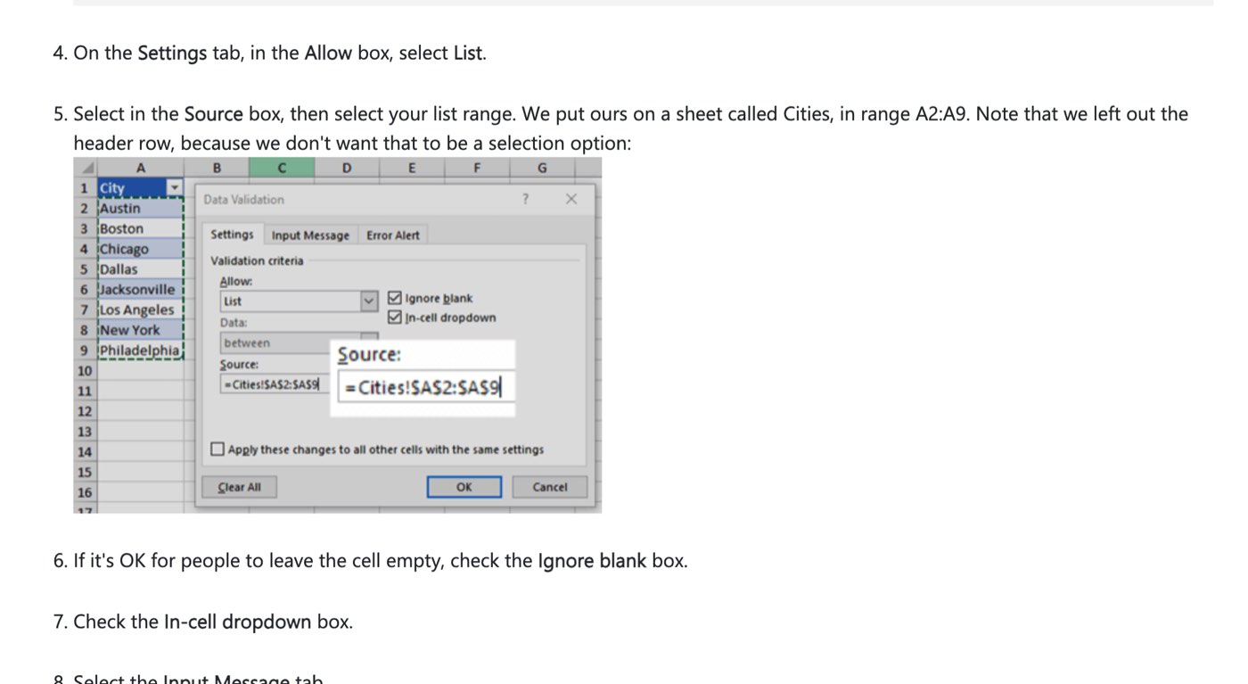
The Data Validation dialog, as shown on Microsoft's support page on September 27, 2026. Allow is set to List and the Source points at a range on another sheet, with the header row left out.
Two optional tabs in the same dialog are worth a look. Input Message shows a note when someone selects the cell, and Error Alert decides what happens when they type something that isn't on the list. Stop refuses the entry; Warning and Information let it through with a message. If you want the list to be a suggestion rather than a rule, pick Warning.
On a Mac
The dialog is the same, and the steps differ only in the labels. On the Data tab, click Data Validation (some versions say Validate), set the Allow pop-up menu to List, then click in Source and select your options. The dialog shrinks while you select; press Return or click the expand button to bring it back, then click OK.
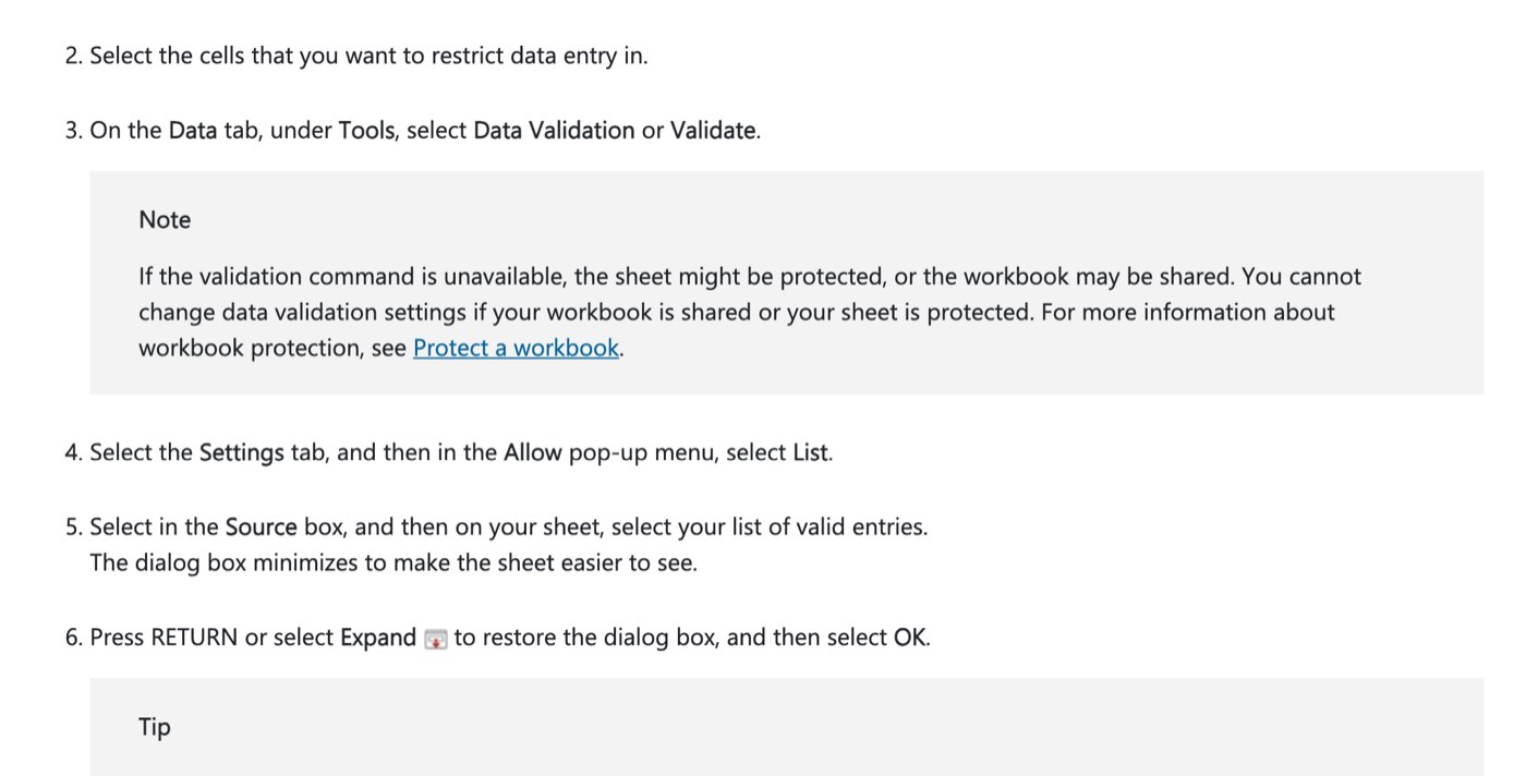
Microsoft's steps for Excel for Mac, captured September 27, 2026. The note explains the most common reason the command is grayed out: a protected sheet or a shared workbook.
In Excel for the web (free)
You don't need a paid copy of Excel. Excel for the web is free with a Microsoft account, as long as the file lives in OneDrive, and it has data validation. On the Data tab, choose Data Tools, then Data Validation, and the rest matches the Windows steps above. The only wording change is in the two optional tabs, which are called Show message and Show Alert.
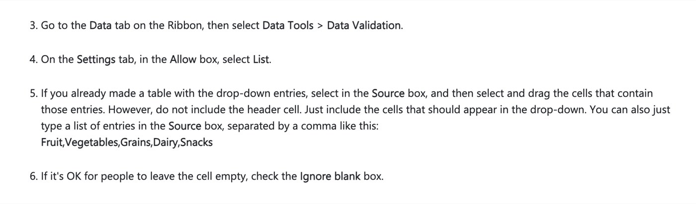
Microsoft's steps for Excel for the web, captured September 27, 2026. Step 5 shows both ways to fill the Source box: select the cells, or type the entries with commas and no spaces.
How do you make the list update itself?
A drop-down built from a plain range is frozen. Add a fifth option under the four you selected and the list still shows four. The fix is to put the options in an Excel table before you build the list.
Click any cell in your column of options and press Ctrl+T (Cmd+T on a Mac). Tick "My table has headers" if the first cell is a heading.
Set up Data Validation as above, and in Source, select the table's cells with the mouse, without the header.
Now type a new option in the row under the table and it joins the drop-down. Microsoft's own description: "as you add or remove items from the list, any drop-downs you based on that table will automatically update". Delete a row from the table and it leaves the list the same way.
Or give the range a name
A named range is a label for a block of cells. Select your options, click in the Name Box (the box at the left end of the formula bar), type a name such as StatusList, and press Enter. In the Source box you can then type =StatusList. Names can't contain spaces, and the same name works from any sheet in the workbook, which is what makes named ranges the basis for the dependent lists below. Microsoft's guide to names covers the rules.
How do you edit a drop-down list?
It depends on where the list came from. Microsoft's editing guide gives one method for each:
Table: add or delete rows in the table. Nothing else to do.
Named range: add the options to the sheet, then open Formulas, Name Manager, pick the name, and reselect the cells in the Refers to box.
Range of cells: add the options, select a cell with the list, open Data Validation, click in Source and reselect the range. Tick "Apply these changes to all other cells with the same settings" so you fix every cell at once.
Typed list: open Data Validation and edit the text in the Source box.
How do you make one list depend on another?
A dependent drop-down shows options that depend on an earlier choice: pick "Fruit" in column A and column B offers apples and pears; pick "Dairy" and it offers milk and cheese. It takes one named range per category and one function.
Put the categories in one column: Fruit, Dairy, Bakery. Build a normal drop-down from them in A2.
For each category, list its items in their own column and name that range exactly as the category is spelled: the fruit column becomes
Fruit, the dairy columnDairy. Use the Name Box for each.Select B2, open Data Validation, set Allow to List, and in Source type
=INDIRECT(A2).
INDIRECT "returns the reference specified by a text string", so when A2 says Fruit, the second list reads the range named Fruit. Two rules keep it working: the names must match the category text exactly, and since names can't contain spaces, a category like "Soft drinks" needs a name like Soft_drinks and a Source of =INDIRECT(SUBSTITUTE(A2," ","_")). If the second list is empty, one of those two rules is the reason.
How do you create a drop-down list with multiple selections?
You can't, with a standard drop-down. A data validation list allows one selection per cell, and Excel still has no setting to change that. What you can do is record several choices another way, covered below.
The question is a live one because of what Microsoft announced on September 24, 2026: for the first time, a cell can hold several values. In the Microsoft 365 Insider announcement, you create such a list with Insert, List or Ctrl+J, then type items separated by commas, and each item stays separately filterable.
It is a preview for Beta Channel only, on Windows Version 2610 (Build 20520.20000) or later and Mac Version 16.114 (Build 26092111) or later, and Microsoft's list of known limitations includes this line: "Data validation can't use a list or array as dropdown items." So it isn't a multi-select drop-down yet, and Microsoft says not to rely on the preview in important workbooks.
Until that changes, the built-in ways to record more than one choice are:
One column per option with checkboxes. In newer versions of Excel for Microsoft 365, select the cells and choose Insert, Checkbox. Each box holds TRUE or FALSE, so formulas can count them.
Several drop-down columns (Choice 1, Choice 2, Choice 3) that all use the same list.
The multi-select drop-downs you see in tutorials are built with a VBA macro. That works on Windows and Mac but not in Excel for the web, and it is outside this guide.
How do you customize a drop-down list?
The list itself has almost no styling options, so the customising happens around it.
Color by choice. Select the cells, then on the Home tab choose Conditional Formatting, Highlight Cells Rules, Text that Contains, type an option such as Done, and pick a fill. One rule per option turns a status column into a color-coded one. The steps are on Microsoft's conditional formatting page.
Bigger text in the list. There is no font setting for the drop-down, so zoom the sheet with the slider at the bottom right. The list scales with it.
Find options by typing. In Excel for Microsoft 365, start typing in the cell and the list narrows to matching items, including matches in the middle of a word. Microsoft calls this AutoComplete for dropdown lists.
Open the list from the keyboard. Press Alt+Down Arrow on Windows, or Option+Down Arrow on a Mac, in a cell that has a list.
How do you remove a drop-down list?
Select the cell or cells (hold Ctrl to pick several), open Data, Data Validation, click Clear All on the Settings tab, and click OK. The values already in the cells stay.
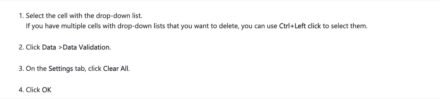
Microsoft's steps for removing a drop-down list, captured September 27, 2026.
To find every drop-down on a sheet when you don't know where they are, press Ctrl+G, click Special, choose Data validation and All, then clear them in one go. That tip is from Microsoft's page on removing lists.
Why isn't your drop-down list working?
No arrow. The arrow only appears when the cell is selected. If it's missing then, open Data Validation and tick In-cell dropdown.
Data Validation is grayed out. The sheet is protected or the workbook is shared, per Microsoft's note on the Mac steps above. Unprotect the sheet or stop sharing, then try again.
The list vanished from some cells. Pasting into a cell replaces everything about it, validation included. Paste values only (Paste Special, Values) to keep the list.
The list shows blank entries. The source range includes empty cells. Shrink the range, or switch to a table so the range is exactly the list.
The dependent list is empty. The name doesn't match the first list's text exactly, or the text contains a space. See the naming rules above.
The header is one of the options. The Source range starts one row too high.
Frequently asked questions
Can the list of options live on a different sheet?
Yes. Click in the Source box, switch to the other sheet and select the cells there. Microsoft's own example keeps the options on a sheet called Cities. A named range makes the reference easier to read.
Does Excel for the web support drop-down lists?
Yes. Data Validation is under Data, then Data Tools, and it is free with a Microsoft account. Macros are the one thing missing, which rules out macro-based multi-select lists there.
Can I use a drop-down list in a formula?
The cell just holds the chosen text, so any formula can read it. =COUNTIF(C:C,"Done") counts how many rows are marked Done.
Is there a shortcut to open the drop-down?
Alt+Down Arrow on Windows and Option+Down Arrow on a Mac open the list in the selected cell.
Why does typing an option give an error?
The Error Alert is set to Stop and the text doesn't match an option exactly, including spaces and spelling. Pick from the list, or set the alert to Warning if near-matches should be allowed.
How this guide was checked
The steps come from Microsoft's support pages for Excel on Windows, Mac and the web, read on September 27, 2026, and the screenshots are of those pages. There is no example workbook to download, because each example above is quicker to build from a blank sheet than to adapt from someone else's file, and building it is how the steps stick. The details on lists in a cell and the data validation limitation come from Microsoft's own announcements of September 24, 2026. This guide is from the Writeouts Tech Desk and follows our editorial standards.
The Writeouts editorial desk for everyday tech: guides and comparisons of AI tools, social media tools and the software people use to get work done. From the Writeouts editorial team.
See everything by @tech-desk
0 comments
Sign in to join the discussion.
Loading comments…