XLOOKUP vs VLOOKUP comes down to this: XLOOKUP does everything VLOOKUP does with fewer mistakes, because it matches exactly by default, can return a column to the left, survives inserted columns and has a built-in "not found" value. VLOOKUP's one remaining advantage is that it works in every version of Excel ever made, while XLOOKUP needs Excel 2021, Excel 2024 or Microsoft 365.
This guide shows each difference with the same small table and the same formulas, calculated side by side on November 11, 2026, so you can see the actual answers rather than take them on trust. It also answers the four questions Google shows under this search: when to use XLOOKUP, how to write one, what the four lookup functions are, and what XLOOKUP's disadvantage is. The last one has a first-hand answer, because the Excel on the test machine couldn't run it.
XLOOKUP vs VLOOKUP at a glance
Behaviour | VLOOKUP | XLOOKUP |
|---|---|---|
Default match | Approximate, unless you add | Exact |
Return a column to the left of the lookup column | No | Yes |
How you name the return column | A number counted from the first column | A range, so inserting columns can't break it |
Value when nothing matches |
| Your own text, as the fourth argument |
Return several columns from one formula | No | Yes, it spills across cells |
Find the last match instead of the first | No | Yes, |
Approximate match on unsorted data | Wrong answers unless sorted | Works unsorted (next smaller or next larger) |
Wildcards | Yes, in exact mode | Yes, with |
Look across a row | No, that is HLOOKUP | Yes, same function |
Binary search for very large tables | Only via approximate mode on sorted data |
|
Works in Excel 2016 and 2019 | Yes | No, shows |
Works in Google Sheets and LibreOffice | Yes | Yes (Sheets since 2022, LibreOffice since 24.8) |
The syntax of each
From Microsoft's VLOOKUP page and XLOOKUP page:
=VLOOKUP(lookup_value, table_array, col_index_num, [range_lookup])
=XLOOKUP(lookup_value, lookup_array, return_array, [if_not_found], [match_mode], [search_mode])
VLOOKUP takes one block of cells and a column number inside it. XLOOKUP takes two separate ranges, the column to search and the column to return, which is the root of most of its advantages. The three optional XLOOKUP arguments are where the extra behaviour lives:
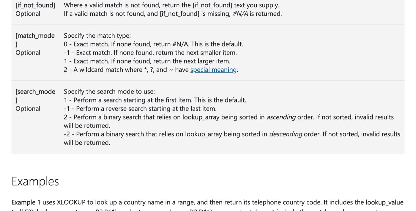
The optional XLOOKUP arguments as Microsoft documents them, captured on November 11, 2026. match_mode 0 is the default, which is why XLOOKUP matches exactly unless told otherwise.
The table every example uses
A sheet named Data, six products, IDs sorted, prices not:
A | B | C | D | |
|---|---|---|---|---|
1 | ID | Product | Category | Price |
2 | 101 | Keyboard | Accessories | 25 |
3 | 102 | Monitor | Displays | 180 |
4 | 103 | Mouse | Accessories | 15 |
5 | 104 | Laptop | Computers | 950 |
6 | 105 | Webcam | Accessories | 40 |
7 | 106 | Headset | Audio | 60 |
Every formula below was put in a workbook with no stored results and calculated by LibreOffice Calc 26.8.2, which implements XLOOKUP with the same arguments as Excel; the reason it wasn't Excel is explained in the testing section. The results are printed exactly as calculated.
What is the difference between XLOOKUP and VLOOKUP?
1. XLOOKUP matches exactly by default. VLOOKUP guesses.
=XLOOKUP(103,Data!A2:A7,Data!B2:B7)   → Mouse
=VLOOKUP(103,Data!A2:D7,2,FALSE)   → Mouse
Both find the mouse, but VLOOKUP needed the FALSE at the end. Leave it off and VLOOKUP switches to approximate matching, which assumes the first column is sorted and returns the largest value that is not bigger than what you asked for. Ask for an ID that does not exist:
=VLOOKUP(107,Data!A2:D7,2)        → Headset
=VLOOKUP(107,Data!A2:D7,2,FALSE)  → #N/A
=XLOOKUP(107,Data!A2:A7,Data!B2:B7)      → #N/A
There is no product 107. VLOOKUP without the fourth argument answered Headset anyway, the row for 106, with no error. That is the mistake that makes VLOOKUP dangerous: a confident wrong answer in a column of hundreds, which nobody notices until the numbers are wrong. The exact-match VLOOKUP and the plain XLOOKUP both returned #N/A, which is what you want when the ID is missing.
2. XLOOKUP has a built-in "not found" value
=XLOOKUP(107,Data!A2:A7,Data!B2:B7,"Not found")   → Not found
=IFERROR(VLOOKUP(107,Data!A2:D7,2,FALSE),"Not found")   → Not found
The fourth XLOOKUP argument replaces the #N/A. VLOOKUP needs an IFERROR wrapped around it, which also hides every other error the formula might raise, such as a broken reference.
3. XLOOKUP can look left
=XLOOKUP("Mouse",Data!B2:B7,Data!A2:A7)      → 103
=VLOOKUP("Mouse",Data!A2:D7,1,FALSE)      → #N/A
=INDEX(Data!A2:A7,MATCH("Mouse",Data!B2:B7,0))   → 103
Given a product name, find its ID. The ID sits to the left of the name, and VLOOKUP can only return columns to the right of the one it searches, so it has no way to do this; the attempt above searched column A for "Mouse" and found nothing. Before XLOOKUP, the answer was INDEX and MATCH, which works but takes two functions to say one thing.
4. XLOOKUP names the return column by its cells, not by a number
VLOOKUP's col_index_num counts columns from the left edge of the table. In =VLOOKUP(103, A2:D7, 4, FALSE) the 4 means Price. Insert a column between B and C and Price becomes column 5, but the 4 in the formula does not change, so the formula now returns Category. Excel adjusts cell references when columns move, and XLOOKUP's return_array is a cell reference: Data!D2:D7 becomes Data!E2:E7 on its own and keeps returning the price. This is the difference that matters most on a shared workbook that other people edit.
5. XLOOKUP can return several columns at once
=XLOOKUP(104,Data!A2:A7,Data!B2:D7) → Laptop, Computers, 950One formula, three answers, filling the three cells to its right. In Excel this spills automatically; in LibreOffice it has to be entered as an array formula (its help page says so), which is how the test entered it. VLOOKUP returns one cell, so three columns means three formulas with three column numbers to keep right.
6. XLOOKUP can find the last match
=XLOOKUP("Accessories",Data!C2:C7,Data!B2:B7)         → Keyboard
=XLOOKUP("Accessories",Data!C2:C7,Data!B2:B7,,0,-1)   → Webcam
Three products are accessories. The default search runs top to bottom and stops at the first, Keyboard; search_mode of -1 runs bottom to top and finds Webcam. VLOOKUP always returns the first match, so "the most recent entry for this customer" needs a helper column or a different approach.
7. XLOOKUP does approximate matches on unsorted data
=XLOOKUP(100,Data!D2:D7,Data!B2:B7,,-1)   → Headset
=XLOOKUP(100,Data!D2:D7,Data!B2:B7,,1)    → Monitor
=VLOOKUP(100,Data!D2:D7,1,TRUE)             → 25
The question is "which product costs 100, or the nearest below it?" Prices in column D run 25, 180, 15, 950, 40, 60, in no order. XLOOKUP with match_mode of -1 scanned them all and answered Headset, at 60, the closest price under 100; with 1 it answered Monitor, at 180, the closest above. VLOOKUP's approximate mode relies on a binary search that assumes the column is sorted, and on this unsorted column it returned 25, which is not the right answer to either question. Microsoft's page says as much: sort the first column or VLOOKUP "may not give the correct value".
8. Both support wildcards
=XLOOKUP("Mon*",Data!B2:B7,Data!D2:D7,,2)   → 180
=VLOOKUP("Mon*",Data!B2:D7,3,FALSE)       → 180
"Mon*" matched Monitor in both. VLOOKUP accepts * and ? whenever it is in exact mode; XLOOKUP needs match_mode of 2, otherwise the asterisk is treated as a literal character. Not a difference in capability, just in where the switch is. For patterns beyond those two wildcards, Microsoft 365 has REGEXTEST and REGEXEXTRACT, whose syntax is covered in the regex cheat sheet.
9. XLOOKUP looks across rows too
=XLOOKUP("Price",Data!A1:D1,Data!A4:D4)   → 15
=HLOOKUP("Price",Data!A1:D7,4,FALSE)       → 15
Give XLOOKUP a row to search and a row to return and it behaves like HLOOKUP, so there is one function to learn instead of two. Nest two of them for a two-way lookup, a product by ID and a column by its header:
=XLOOKUP("Price",Data!A1:D1,XLOOKUP(104,Data!A2:A7,Data!A2:D7)) → 95010. XLOOKUP has a binary search mode
=XLOOKUP(105,Data!A2:A7,Data!B2:B7,,0,2) → Webcamsearch_mode of 2 (ascending) or -2 (descending) uses a binary search, which is much faster on a table of hundreds of thousands of rows, but only if the lookup column is sorted that way; Microsoft's documentation says unsorted data gives "invalid results". The IDs here are sorted, so it found the webcam. For an ordinary table, leave search_mode out.
Three things that trip up both functions
=XLOOKUP("mouse",Data!B2:B7,Data!A2:A7)   → 103
=XLOOKUP(102,Data!A2:A7,Data!E2:E7)      → 0
=VLOOKUP(102,Data!A2:E7,5,FALSE)        → 0
Neither function cares about case: "mouse" found Mouse. Both return 0 when the matched cell is empty, rather than an empty cell: looking up ID 102 in the empty column E gave 0 from each. Append & "" to the formula when a blank should stay blank.
The third is the usual cause of a #N/A against an ID that is visibly there: in Excel, the text "103" is not the number 103. Microsoft's #N/A troubleshooting page lists it first: "the lookup value and the source data are different data types", typically after a paste from another system. Convert one side with VALUE() or TEXT(). This is one place LibreOffice Calc differs from Excel: in the test run, =XLOOKUP("103",Data!A2:A7,Data!B2:B7) and the VLOOKUP equivalent both matched the number and returned Mouse, so those two results are Calc's, not Excel's.
When should you use XLOOKUP?
Whenever everyone who will open the workbook has Excel 2021, Excel 2024 or Microsoft 365, including Excel for the web and the phone apps. That covers most offices in 2026, and Microsoft's own VLOOKUP page now opens with a tip to try XLOOKUP instead.

Microsoft's VLOOKUP page on November 11, 2026 steers readers to XLOOKUP before it explains VLOOKUP.
Use it in particular when the lookup column is not the first column, when other people insert columns in the table, when a missing value should show a message rather than #N/A, when you need the last match, or when you need several columns from one row.
When is VLOOKUP still the better choice?
Someone opens the file in Excel 2016 or 2019. Every XLOOKUP cell shows
#NAME?there, and recalculating the sheet wipes the stored results. If a file goes to a client or a supplier whose Excel you don't know, VLOOKUP is the safe choice.Templates and macros built around VLOOKUP. Rewriting working formulas for their own sake is risk without reward; convert when you touch them for another reason.
Other tools that read Excel formulas. Some reporting and import tools evaluate only the older function set. Check before you convert a file they consume.
There is no case where VLOOKUP gives a better answer than XLOOKUP. The reasons to keep it are all about who else has to open the file.
What is the disadvantage of XLOOKUP?
Availability. XLOOKUP exists only in Excel 2021, Excel 2024, Microsoft 365, Excel for the web and the mobile apps. Open a workbook that uses it in Excel 2016 or Excel 2019 and the cells show #NAME?.

Microsoft's own note on availability, captured on November 11, 2026.
That is not a theoretical problem. The Mac this article was tested on has Excel version 16.114.4 installed, and when the test formulas were entered into it, =XLOOKUP("world",A1:A2,A1:A2) came back as #NAME?. So did LET, FILTER, XMATCH and TEXTSPLIT, and even IFS and CONCAT; VLOOKUP and LEN worked. Version 16 covers every Excel for Mac since 2016, so the number alone does not tell you which functions you have; the licence does. If you are not sure, type =XLOOKUP( in a cell and see whether Excel offers to complete it.
Two smaller disadvantages. A multi-column XLOOKUP spills into neighbouring cells and shows #SPILL! if one of them is occupied. And the binary search modes return wrong answers on unsorted data without an error, so use them only on a column you know is sorted.
How do I do an XLOOKUP in Excel?
Click the cell where the answer should appear and type
=XLOOKUP(.Type or click the value to look up, then a comma. For an ID in cell F2:
F2,Select the column that holds the IDs, then a comma:
Data!A2:A7,Select the column that holds the answers:
Data!B2:B7. For several columns select them all,Data!B2:D7, and the result spills to the right.Optionally add what to show when there is no match:
,"Not found".Press Enter. The whole formula reads
=XLOOKUP(F2,Data!A2:A7,Data!B2:B7,"Not found").
Leave match_mode and search_mode out unless you need a nearest match, a wildcard, the last match or a binary search. If the lookup column is in a table, use the structured name, such as Products[ID], and the range grows with the table, the same trick that keeps an Excel drop-down list up to date.
What are the four types of lookup in Excel?
Function | Searches | Status |
|---|---|---|
| Down the first column of a table, returns from a column to its right | Still supported everywhere |
| Along the first row of a table, returns from a row below | Still supported; Microsoft's page suggests XLOOKUP |
| A single row or column, approximate match only, sorted data | Kept for compatibility |
| Any row or column, returns from any row or column | Excel 2021 and later |
Two more belong in the same conversation. INDEX with MATCH is the pre-2019 way to look left and to survive inserted columns, and it still works in every version. XMATCH, released alongside XLOOKUP, returns the position of a match with the same match and search modes, for when you need the row number rather than a value.
Does XLOOKUP work in Google Sheets and LibreOffice?
Yes to both, with the arguments in the same order. Google Sheets names the first three search_key, lookup_range and result_range, calls the not-found value missing_value, and uses the same mode numbers for match_mode and search_mode. LibreOffice Calc added XLOOKUP in version 24.8 and, unlike Excel, needs a multi-cell result entered as an array formula.
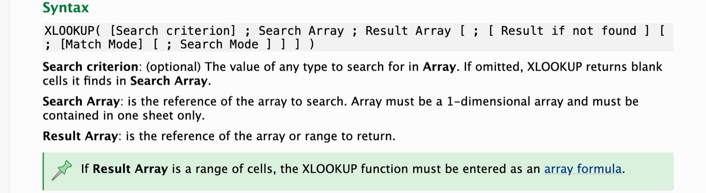
LibreOffice's XLOOKUP help on November 11, 2026. Same arguments as Excel, semicolons between them, and the array-formula rule for multi-cell results.
A workbook that uses XLOOKUP can therefore move between Excel, Sheets and Calc without rewriting, which was not true of newer Excel functions for a long time.
How this was tested
The six-row product table and all 27 formulas printed above were written into a workbook with no stored results, by a script, so nothing could be typed wrong. The intention was to calculate them in Excel for Mac 16.114.4 on an Apple M2 Mac. That copy of Excel returned #NAME? for XLOOKUP and every other function newer than Excel 2016, as the disadvantage section describes, so the same workbook was calculated by LibreOffice Calc 26.8.2, run headless from its downloaded disk image on November 11, 2026, and the values it saved were read back by script. The multi-column lookup was entered as an array formula, which Calc requires.
Calc's XLOOKUP follows Microsoft's argument list and mode numbers, and the results printed match the behaviour Microsoft's documentation describes for each case, with two exceptions the text points out where they appear: the approximate VLOOKUP on an unsorted column, which depends on each program's search, and text-versus-number matching, where Calc is lenient and Excel is not. The workbook, the generator script and the recorded results are kept with the article so the run can be repeated in Excel by anyone whose licence includes XLOOKUP.
Frequently asked questions
Is XLOOKUP faster than VLOOKUP?
On ordinary tables neither is slow enough to notice. On very large sorted tables, XLOOKUP's binary search mode (search_mode 2) and VLOOKUP's approximate mode both use a binary search and are far faster than an exact scan. No timing was done for this article, so no number is claimed.
Can XLOOKUP replace INDEX MATCH?
Yes, for every common use: looking left, surviving inserted columns, two-way lookups and last-match searches. INDEX/MATCH is still worth knowing because it works in Excel 2016 and 2019 where XLOOKUP does not.
Why does XLOOKUP return #N/A?
Because nothing in lookup_array equals lookup_value. The usual causes are a number stored as text on one side (the "103" test above), trailing spaces, or searching the wrong column. Add a fourth argument to show a message instead of the error.
Why does XLOOKUP show #NAME?
That Excel does not have the function: Excel 2016, Excel 2019, or a copy whose licence does not include it. The formula is fine; the program is the limit. VLOOKUP or INDEX/MATCH will work there.
Is VLOOKUP going away?
No. Microsoft's VLOOKUP page lists it as applying to Excel for Microsoft 365, Excel 2024, 2021, 2019 and 2016, and every spreadsheet program supports it. It is simply no longer the best tool when XLOOKUP is available.
Does XLOOKUP work in Excel 2019?
No. Microsoft states that XLOOKUP is not available in Excel 2016 and Excel 2019. It arrived with Excel 2021 and Microsoft 365.
The Writeouts editorial desk for everyday tech: guides and comparisons of AI tools, social media tools and the software people use to get work done. From the Writeouts editorial team.
See everything by @tech-deskEdited by Rajat Chauhan. How articles here are written and edited.
0 comments
Sign in to join the discussion.
Loading comments…